Quantum Computer Algorithms: Part 2 - Amplitude Amplification
by Dave D'Rave
In the academic literature of quantum algorithms, you will often encounter a class of functions called "the oracle."
These are gate sets which (potentially) have a large number of inputs and only one output, such that the output is interpreted as either being "Yes" or "No." In the formalism, there are n active inputs, plus an input which has been set to |0⟩, and the oracle operates by performing a conditional-NOT on the |0⟩ input, which may cause it to become non-zero.
As a practical matter, what usually happens is that the controlled-NOT is subject to some superposition of states, and that the output is something like: k (|0⟩ + 0.00001 |1⟩)
This can become large and complicated.
For example, let's say that you have a (classical) oracle which is mining Bitcoin. You give it the current working block and a 32-bit nonce. The output will be "1" if the output hash is below the threshold, and a "0" otherwise.
Strictly speaking, if you have a quantum oracle doing the same thing, it will produce the same results, which is kind of pointless.
More interesting is if I build a quantum Bitcoin oracle, and then send it the current working block and a superposition of, say, 64 nonce values. The output will then either be |0⟩, if none of the proposed nonce values is good, or (0.992 |0⟩ + 0.125 |1⟩), if one of the nonce values is good and the others are bad. (For now, we are not interested in cases where more than one nonce is good.)
This looks like a step forward, in that we now have a factor of 64 reduction in work. The problem is that it is not easy to tell the difference between a |0⟩ output state and a non-zero output state.
Multiple Measurements: An Inefficient Way to Measure Superpositions
If you think that you have a qubit in the |one-sixty-fourth⟩ state, the obvious way to proceed is to measure the system output, then run the algorithm again, measure it again, etc. This takes a lot of time and effort, and does not guarantee that you will ever get an exact measurement. You will get an asymptotic approach to the answer.
What we really want is a function which takes in |0⟩ and returns |0⟩, but which returns |1⟩ when it is given a mixed state. This sort of thing is called "amplitude amplification," and is not available in a clean, easy-to-use quantum operator.
The closest approximation to an operator which amplifies an arbitrary ket is something which accepts an input which is either |0⟩ or, say, |0.7⟩. (Note that this is not necessarily a superposition: The input ket is either |0⟩ or |0.7⟩.)
A Differential Operator for Amplitude Amplification
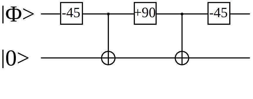
This operator is intended to return |0⟩ if the |Φ⟩ input is equal to |0⟩ and to return |1⟩ if the |Φ⟩ input is equal to |0.7⟩.
The two possible input cases look like this:
1.)
2.)
- If the |Φ⟩ input is equal to |0⟩, then the first rotation operator will make it equal to |-45°⟩, or |-0.7⟩. The first C-NOT will change the output qubit to |-45°⟩.
- The second rotation operator will make |Φ⟩ is equal to |+45°⟩, or |0.7⟩. The second C-NOT will make the output qubit equal to |0⟩.
- The third rotation operator will cause the input qubit to return to its original value.
- If the |Φ⟩ input is equal to |0.7⟩, then the first rotation operator will make it equal to 0°, or |0⟩. The first C-NOT will do nothing.
- The second rotation operator will make |Φ⟩ is equal to |1⟩. The second C-NOT will make the output qubit equal to |1⟩.
- The third rotation operator will cause the input qubit to return to its original value.
This class of quantum operator is called "a differential operator" because it is designed to have two different controlled-operators in the output path, such that some of the control input sets will exactly cancel out the two changes in the output path. In this case, if the |Φ⟩input is equal to |0⟩, then the two C-NOT operators will cancel out, and the output will be equal to |0⟩.
By design, some of the control input sets will not cancel out. In this case, a control input of |0.7⟩ will cause the output to be equal to |1⟩, which is often useful.
Variant Differential Operators
In the academic literature, the controlled-NOT gate is commonly used to build a differential operator, but practical quantum logic often prefers to use things like controlled-rotate or controlled-reflect.
In particular, gates like "Controlled-Rotate-by-90-Degrees" or "Controlled-Rotate-by-11.25-Degrees" simplify the part count of certain algorithms. These methods can also reduce the circuit's susceptibility to noise.
One commonly encountered controlled-reflect is "Controlled Hadamard." This is pretty much what it sounds like: It is a Hadamard gate with a control input.
If you look closely at questions like "How do i make a Toffoli gate out of 2-input blocks," you will find yourself looking at "Controlled-U Gates," where the term "U Gate" describes either a generic gate or a "Universal Gate."
In the literature of quantum computer engineering, exotic types of gates are often used because they have some kind of cost advantage or noise advantage. This is similar to how most of the current mass-produced chips are built out of NAND gates, even though the "Intro to Computer Architecture" classes only talk about AND, OR, and NOT gates. The textbooks are not the industry.
Higher-Order Control Values
In order to get the big, impressive speed improvements, practical quantum algorithms will need to reliably operate using superpositions of 256 qubits or 4096 qubits. Equally important, there will often be a need to determine if a given large superposition is in a pure state or not.
For example, if we have a traveling salesman problem involving 256 nodes, then you will need several thousand qubits just to hold the problem set. If your algorithm requires a superposition, such that "Given a superposition of itineraries which start in Node 5, do any of these itinerary costs less than 254,133?", it is likely that the output waveform will have a very low density.
In fact, as the algorithm iterates to the best solution (lowest cost itinerary), you will find yourself looking at output ket values like: k (0.999999 |0⟩ + 0.0000000000001 |1⟩)
Identifying algorithms which can efficiently tell whether such kets are in a pure state is an ongoing research topic.
Notes
This article uses a mixture of qubit labels, which may be confusing.
The main symbols used are "bracket notation," using the standard quantum computer idea of a computation basis. This is a subset of the usual quantum mechanics formalism you may encounter in an "Intro to Quantum Mechanics" class.
The two basis vectors typically used are the kets named |0⟩ and |1⟩.
The most common superposition used in quantum computing books is: k (|0⟩ + |1⟩)
Where k is normalized by the constant 0.707. (This is equal to the square root of one-half, and is also equal to the square root of two divided by 2, and is also equal to the cosine of 45°.) This particular superposition is known variously as |0.707⟩, |+0.7⟩, |45°⟩, |+45°⟩, etc.
In the literature, the two common basis vectors are in the real plane. Advanced quantum computer algorithms require the ability to rotate or reflect vectors into the imaginary plane.
The basis vector in the imaginary plane is often named |+⟩ or |i⟩. Superpositions are sometimes encountered with names like: k |1-i⟩ or k (|1⟩ + |i⟩)
These are called "complex kets" or "complex valued kets."
Finally, it is useful to know that quantum simulators often use the Dirac matrix representation, in which kets are described by a vector. There is a one-to-one mapping between bra-ket notation and Dirac matrix notation.
Quantum Computer Algorithms: Part 1 - Quasi-Classical Methods